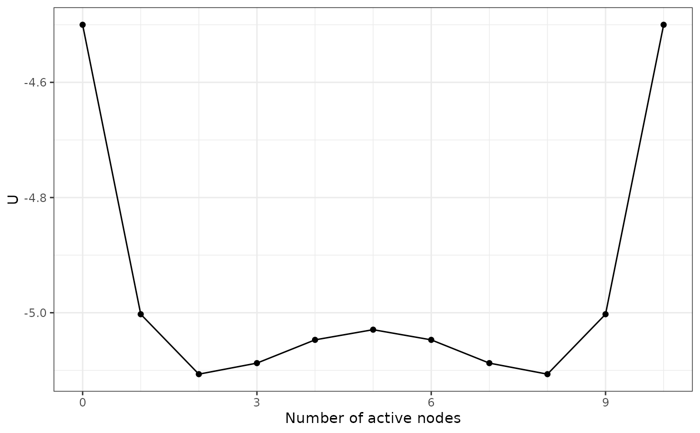
Make a 2D landscape for an Ising network

Calculate the potential value $U(n)$ for each system state, represented by the number of active nodes $n$. The potential value is determined so that the Boltzmann distribution is preserved. The Boltzmann distribution is the basis and the steady-state distribution of all dynamic methods for Ising models, including those used in IsingSampler::IsingSampler() and Glauber dynamics. This means that if you assume the real-life system has the same steady-state distribution as the Boltzmann distribution of the Ising model, then possibility that their are $n$ active nodes in the system is proportional to $e^{U(n)}$. Because of this property of $e^{U(n)}$, it is aligned with the potential landscape definition by Wang et al. (2008) and can quantitatively represent the stability of different system states.

Usage

make_2d_Isingland(thresholds, weiadj, beta = 1, transform = FALSE)

Arguments

thresholds, weiadj: The thresholds and the weighted adjacency matrix of the Ising network. If you have an IsingFit object estimated using IsingFit::IsingFit(), you can find those two parameters in its components (<IsingFit>$thresholds and <IsingFit>$weiadj).
beta: The $\beta$ value for calculating the Hamiltonian.
transform: By default, this function considers the Ising network to use -1 and 1 for two states. Set transform = TRUE if the Ising network uses 0 and 1 for two states, which is often the case for the Ising networks estimated using IsingFit::IsingFit().

Value

A 2d_Isingland object that contains the following components:

dist_raw,dist Two tibbles containing the probability distribution and the potential values for different states.
thresholds,weiadj,beta The parameters supplied to the function.
Nvar The number of variables (nodes) in the Ising network.

Details

The potential function $U(n)$ is calculated by the following equation: $$U(n) = -\log(\sum_{v}^{a(v)=n} e^{-\beta H(v)})/\beta,$$ where $v$ represent a specific activation state of the network, $a(v)$ is the number of active nodes for $v$, and $H$ is the Hamiltonian function for Ising networks.

References

Wang, J., Xu, L., & Wang, E. (2008). Potential landscape and flux framework of nonequilibrium networks: Robustness, dissipation, and coherence of biochemical oscillations. Proceedings of the National Academy of Sciences, 105(34), 12271-12276. https://doi.org/10.1073/pnas.0800579105 Sacha Epskamp (2020). IsingSampler: Sampling methods and distribution functions for the Ising model. R package version 0.2.1. https://CRAN.R-project.org/package=IsingSampler Glauber, R. J. (1963). Time-dependent statistics of the Ising model. Journal of Mathematical Physics, 4(2), 294-307. https://doi.org/10.1063/1.1703954

Examples

Nvar <- 10
m <- rep(0, Nvar)
w <- matrix(0.1, Nvar, Nvar)
diag(w) <- 0
result1 <- make_2d_Isingland(m, w)
plot(result1)